Little Earth / Field Notes / Now With a Sea Floor
GIS & Fabrication
Now With a Sea Floor
I reprinted Vancouver Island. The ocean isn't a flat black slab any more — it's real bathymetry. Six colours, cut into 46 tiles.
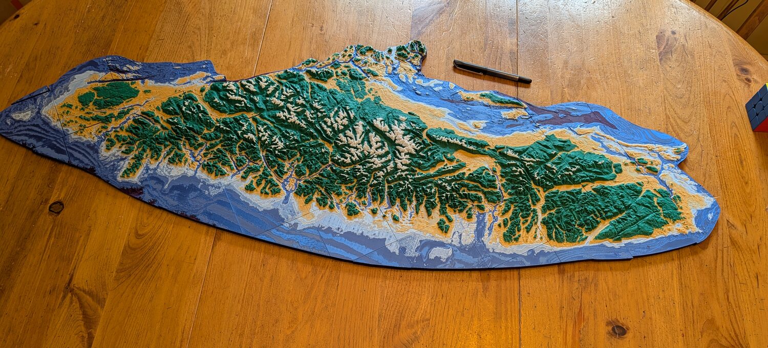
One metre of Vancouver Island, 46 tiles, six colours. The pen is a Sharpie.
Two things bothered me about the Vancouver Island model I printed at the end of 2025. The first was it only had two colours — red land and black ocean. The second was the large areas of flat boring ocean.
So I built it again. Same island, a metre long this time, and the water has depth (bathymetry).
The ocean has a floor now
The sea floor around Vancouver Island turns out to be the more dramatic half of the map. The Strait of Georgia is a proper trench, Juan de Fuca is a channel with sides, and off the west coast the shelf runs out for kilometres before falling off the edge of itself. None of that was in the first model, and a fair amount of it has more relief than anything happening above the waterline.
The land above the waterline comes from the province, via DataBC. Everything below it comes from the Canadian Hydrographic Service, whose licence states in capital letters that the data is for non-navigational use only — a bar I am confident a plastic map at 1:425,000 clears.
Getting them into the same file meant merging two rasters that disagreed about nearly everything. The land data is 25-metre resolution, already projected in metres. The bathymetry is roughly 100-metre, in raw longitude and latitude, and reaches down to −2,895 m. And the two files don't even agree on how to say "no data here": the bathymetry uses 3.4 × 1038, the largest number a 32-bit float can hold, while the land model uses plain zero.
That last one sounds like a problem and is quietly a gift. Because the land data treats 0 m as "nothing to report", every pixel sitting right at the shoreline falls through to the bathymetry underneath — which is exactly where you want the two datasets to hand off to each other. Warp the sea floor onto the land's own 25-metre grid, stack the land on top, and you get one continuous surface running from the bottom of the continental slope to the summit of the Golden Hinde.
The gift has a bill attached, mind. "Zero means nothing here" can't tell the difference between the sea and genuinely flat ground, so the same rule that hands the shoreline over cleanly also punches holes in lakes and low flat country — places the bathymetry knows nothing about either. Those get filled by interpolating outward from whatever data surrounds them, which works right up until a hole is wider than the search radius you gave it. And because the fill doesn't know where to stop, it smears a rind of invented elevation out past the edge of the study area, so the last step is to clip the whole thing back to the boundary and throw that rind away.
The result is a single raster of 17,020 × 12,527 pixels — 213 million of them, 92 million actually carrying an elevation and the rest empty sea outside the boundary — spanning −1,125 m to +2,169 m. That range turns out to matter more than a pair of numbers should, and I'll come back to it.
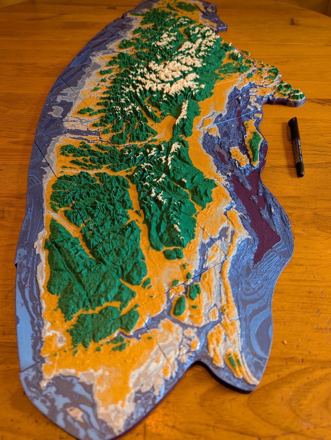
Looking along the island, with the Strait of Georgia on the right. That deep purple trough is geometry the first model didn't know existed.
Six colours, chosen in metres
Last time there was one colour change, at sea level, and engineering it cleanly was the entire point of the exercise. This time there are five, and the useful shift is that I specify them in real-world metres — −350, −50, 0, +200 and +1,100 — and let the tool work out where those land in a model that has been shrunk by a factor of 425,000 and stretched vertically by three.
Six bands come out of five cuts: purple for the deep water, dark blue, then a pale blue shelf, gold for the lowlands, forest green for the mountains, and white on the peaks. That's a hypsometric map, the colour scheme every school atlas uses — except here the colour isn't printed onto the map, it is the material, which means the printer never has to change filament in the middle of a layer.
The subtlety that bites
At three-times vertical exaggeration on a metre-wide island, a single 0.12 mm print layer is about 17 metres of elevation. If the sea-level cut doesn't land exactly on a layer boundary, the slicing software rounds it to the nearest one — and a strip of genuinely dry coastal land gets printed in ocean blue. So the tool snaps every colour threshold onto the slicer's layer grid before it cuts anything.
One program, one file
The first version of this was a QGIS plugin, a Python script, and a JSON config file I had to keep in sync with both by hand. This one is a single program written in Rust. You hand it the elevation data and a boundary polygon; it hands back a print-ready project.
I'll spare you the geometry — the first post covers the core idea and it hasn't changed: you slice the sealed solid into horizontal slabs rather than trying to colour individual triangles. What's changed is everything around it.
- It builds all 46 tiles at once. The island is bigger than the print bed, so it has to come apart into bed-sized squares anyway — and each of those is genuinely independent. Sample the elevation, build a solid, clip it to the boundary I drew around the island, slice it into bands. There's nothing to coordinate, so they just run in parallel, one tile per core. The old workflow was one tile at a time with me in the loop between each one; this one is a single command, and the only thing that takes any real time afterwards is the printing.
- It's one file. No Python, no QGIS, no plugin, nothing to install to run it. Rust compiles to a single self-contained binary per platform, so "installing" it means copying an 8 MB file onto the machine — even the C++ geometry kernel that does the actual cutting is baked into the executable. Merging the two elevation sources in the first place is still a GDAL job, but that happens once, outside the tool.
- It writes a real print project, not a pile of models. Forty-six separate model files means forty-six imports into Bambu Studio, and it helpfully duplicates the entire filament table on each one — and the printer tops out at sixteen, so you're over the line before you're three tiles in. Instead the tool emits one project file with all 46 tiles already arranged across 12 print plates, sharing a single filament table, brim disabled, and the purge tower parked clear of the front-left corner the printer can't reach. Open it and press slice.
And one small vanity: the company URL and logo are stamped into the underside of the tiles, flush with the base so they need no support material — the first 0.6 mm, five layers, of each print. Forty-five of the forty-six got one. The last is a 32 mm-wide sliver of coast, and a 40 mm-wide logo clipped to it leaves nothing at all.
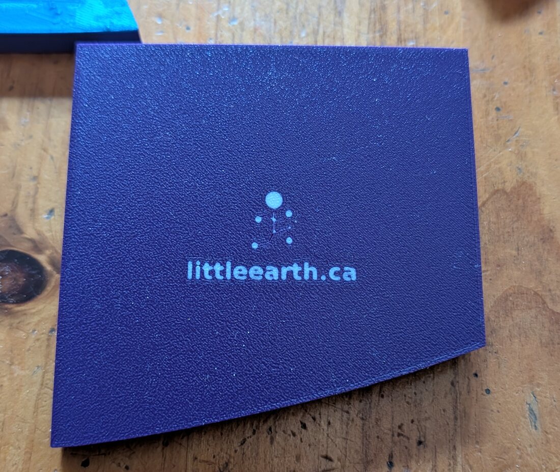
A tile turned over. It's the same white that tops the mountains, so the logo costs no extra colour. The mark is mirrored in the model so it reads the right way round once you flip it — and that curved bottom edge is where the study boundary cut the tile.
That inlay is also the one place my tidy claim about colour breaks down. The six elevation bands are stacked slabs, so they never collide within a layer — but the branding is a separate body sitting alongside the bottom band, which means those first five layers really do swap filament mid-layer. Everything above them doesn't.
Six colours, four slots
The map needs six colours. The automatic changer that feeds the printer — Bambu's AMS — holds four. That arithmetic is how this project ended up justifying a second one: an expense I maintain was driven entirely by the data, and not at all by my having wanted another one anyway.
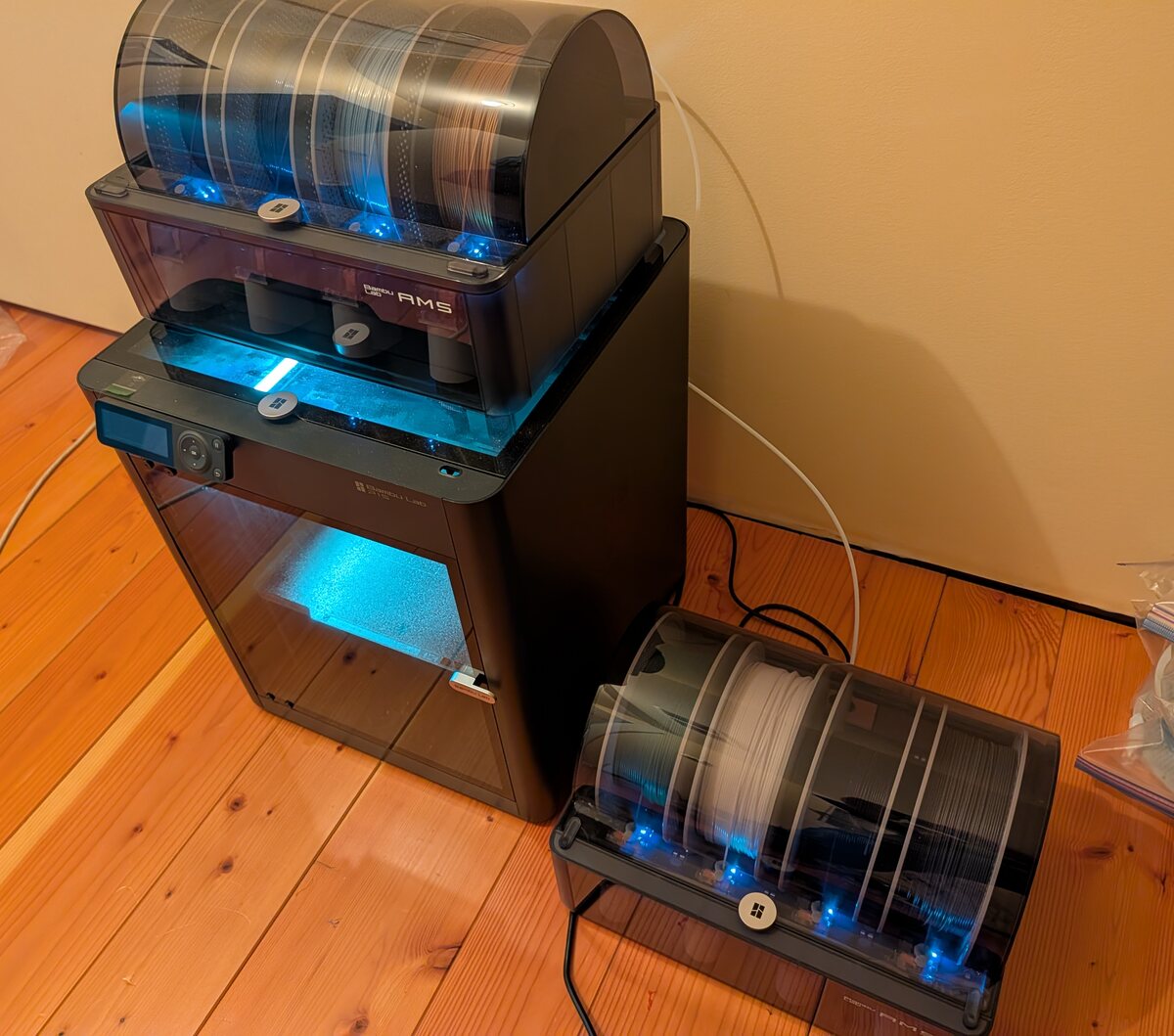
The justification, in hardware: one changer on top, the second one beside it. Eight slots for six colours, and room to grow.
Two things I only found out by printing it
Neither of these was visible on a screen. Both turned up the moment there were tiles on the table — which is the case for making physical objects out of data. The object answers back, and it has no interest in what you intended.
The base isn't where you think it is
I asked for a 3 mm base: the flat pad underneath the terrain that makes the thing solid, printable and flat enough to sit on a table.
What you actually get is a 3 mm base under the lowest point in the entire dataset. And the lowest point in this dataset is 1,125 m down, at the foot of the continental slope off the west coast. At that one pixel the model is exactly 3 mm thick, as ordered, and out across the deep water it stays within a few millimetres of it.
Everywhere else, the thickness is that 3 mm plus however far the sea floor sits above the deepest point. Under the shoreline, that's about 11 mm. Under the summits, 26 mm. Adding the continental slope to the dataset quietly moved the model's floor a kilometre downwards, and every tile got taller.
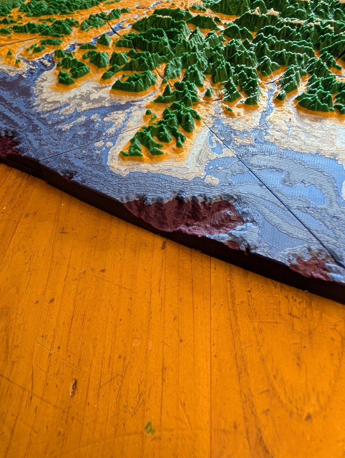
Out past the shelf break the model thins to a few millimetres, bottoming out at exactly 3 mm over the single deepest pixel on the map.
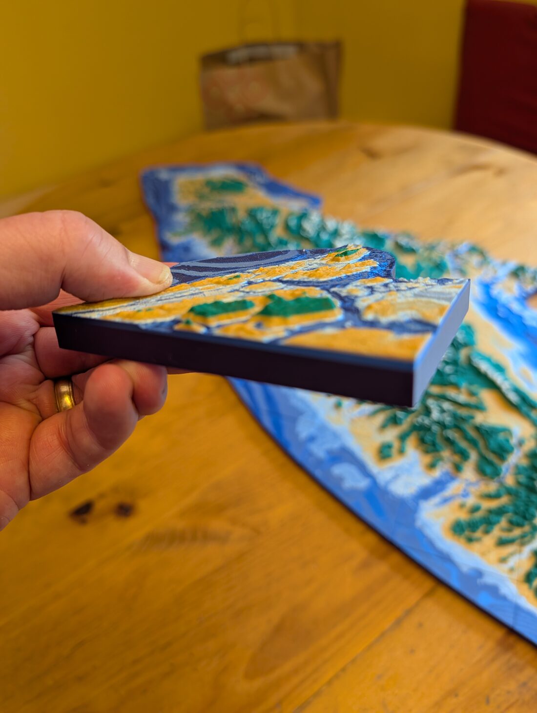
A tile lifted out and turned edge-on: the same 3 mm base, plus eight more millimetres of continental slope underneath it.
I don't hate the result. That purple slab is real information — it's the shape of the sea floor seen edge-on — and it gives the tiles a satisfying heft. But I didn't choose it, and I paid for it in filament I hadn't budgeted for. The fix is to measure the base per tile, or to clamp how deep the model is allowed to go. Both are on the list.
A grid doesn't care about geography
The tiles come from a plain 10 × 8 grid laid over the island. Cells that miss the boundary entirely get dropped, which is worth having — it takes 80 down to 46. But the survivors get cut wherever the grid happens to fall, and sometimes the grid says "here is a 14-millimetre splinter of coastline, print it by itself". The smallest tile in the set is 14 × 34 mm; the next is 63 mm long and 12 mm wide.
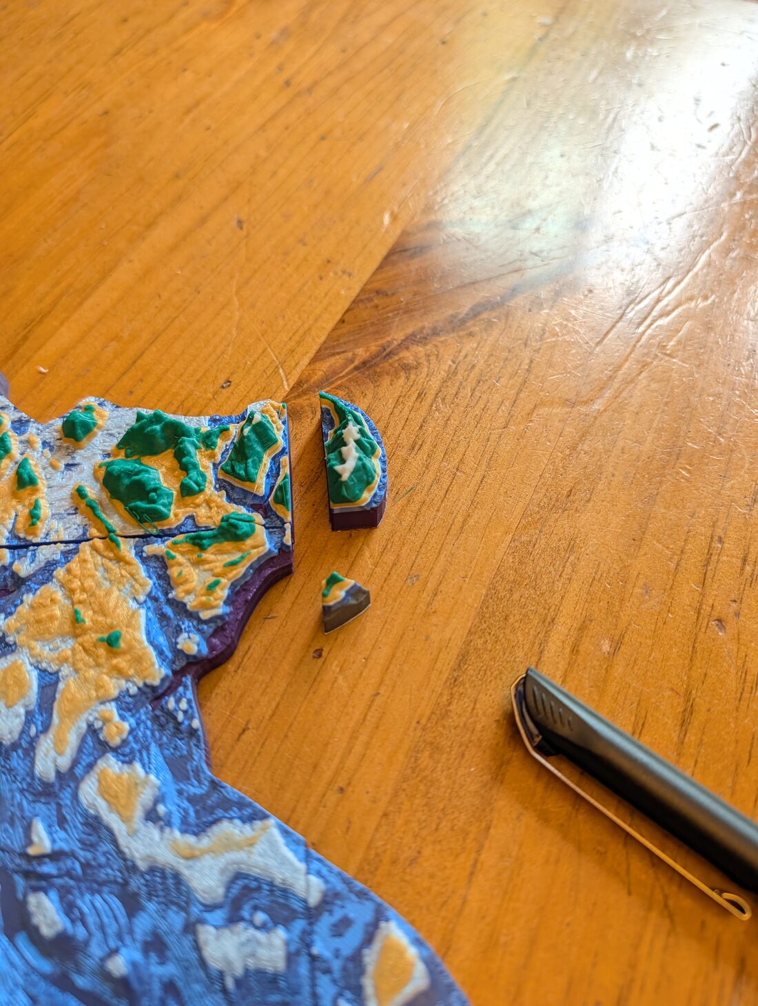
Two of the pieces the grid produced. Both are perfectly valid tiles — watertight, correctly coloured, and thoroughly silly.
They print fine and they fit fine. They're just fiddly to handle, easy to lose under a table, and faintly ridiculous. A smarter chopper would nudge its cuts towards the coastline, or fold a runt into the tile next door. Also on the list.
The numbers
| Measure | Value |
|---|---|
| Assembled size | 1,000 × 736 mm |
| Scale | 1 : 425,000 horizontal, 3× vertical exaggeration |
| Tiles | 46, at 100 mm square, across 12 print plates |
| Source grid | 17,020 × 12,527 px at 25 m — 213 million pixels, 92 million with data |
| Elevation range | −1,125 m to +2,169 m (the Golden Hinde, as a 25 m grid sees it) |
| Colour bands | 6, cut at −350, −50, 0, +200 and +1,100 m |
| Layer height | 0.12 mm — about 17 m of elevation per layer |
| Base | 3 mm under the deepest point |
| Printer | Bambu Lab P1S, 0.4 mm nozzle, PLA |
Resources
- Provincial elevation data — DataBC — the land surface, on a 25 m grid
- Non-Navigational (NONNA) bathymetry — Canadian Hydrographic Service — the sea floor, at roughly 100 m
- GDAL — used outside the tool to merge and gap-fill the two elevation sources
- Rust and Manifold — the language and the geometry kernel behind the slicer
- Bambu Lab P1S
- 3D Printing Vancouver Island — the first attempt, and the geometry in detail
What's next
The base measurement and the grid-versus-coastline problem are the two obvious fixes. After that, the interesting direction is overlays — rivers, roads and trails inlaid as their own colour, using the same trick that puts the logo on the underside. There's also a browser-based terrain project sharing a surprising amount of DNA with this one.