Little Earth / Field Notes / 3D Printing Vancouver Island
GIS & Fabrication
3D Printing Vancouver Island
From a Digital Elevation Model to multi-colour physical terrain using QGIS, Python, and a Bambu 3D printer.
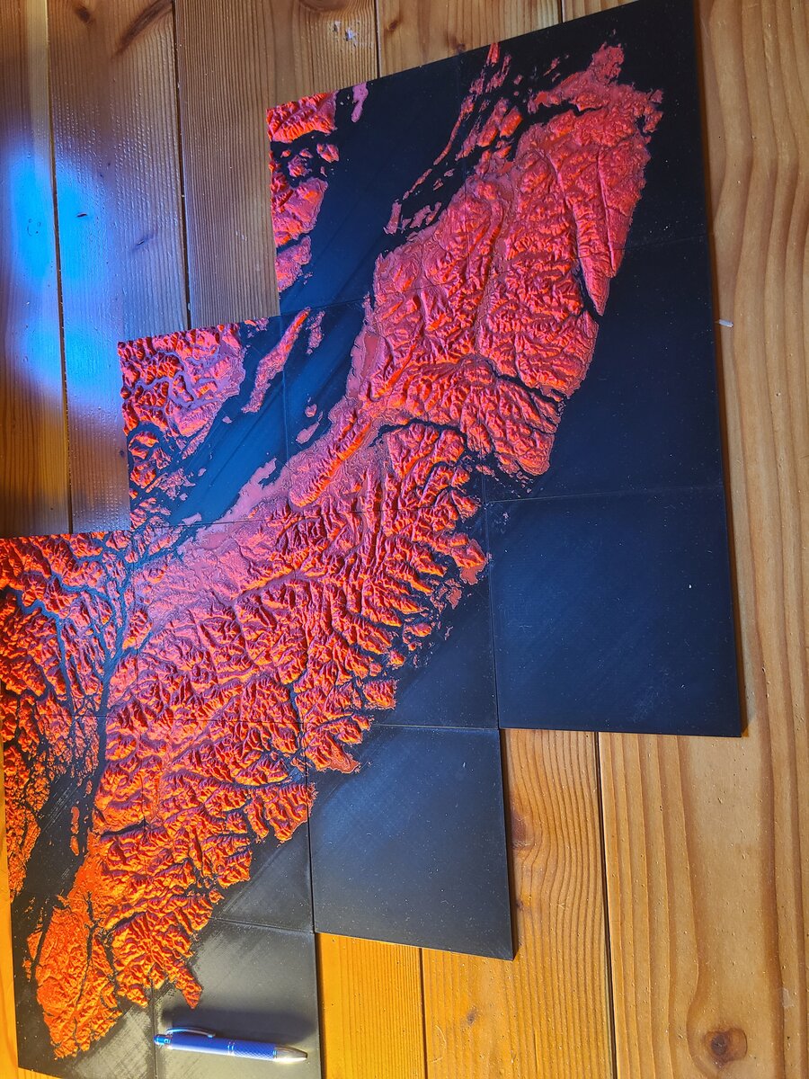
The completed Vancouver Island model: 14 tiles, two colours
The Project
As someone who works with GIS data professionally, I've always wanted to bring digital terrain data into the physical world. Vancouver Island, with its dramatic mountain ranges, intricate coastlines, and deep fjords, seemed like the perfect candidate for a 3D printed terrain model.
The goal was simple: create a physical representation of the island that clearly distinguished land from ocean using two different filament colours. The reality, as usual, was more complex and required writing custom code to solve an interesting geometry problem.
What You'll Learn
This post covers the complete workflow from DEM data to finished print, including the geometry slicing problem I had to solve with Python and trimesh.
The Tools
| Category | Tool | Purpose |
|---|---|---|
| GIS Software | QGIS + DEMto3D Plugin | Convert DEM raster to 3D mesh, tile export |
| Programming | Python 3.11 | Custom mesh processing script |
| 3D Library | trimesh | Mesh loading, boolean operations, export |
| Slicer | Bambu Studio | Prepare print files with material assignments |
| Printer | Bambu Lab P1S + AMS | Multi-colour FDM printing |
| Filament | PLA (Black + Orange) | Ocean and land colours |
Step 1: Acquiring DEM Data
The foundation of any terrain model is the Digital Elevation Model (DEM). For Vancouver Island, I used the High Resolution Digital Elevation Model (HRDEM) from Natural Resources Canada. The island spans roughly 460km north to south, and the HRDEM provides excellent detail while keeping file sizes manageable.
Key elevation statistics from the DEM:
- Lowest point: -220m (Randomly selected to give the print a bit of depth at the bottom)
- Highest point: 2,195m (Golden Hinde, but DEM includes some mainland at 3,111m)
- Sea level: 0m (our target threshold)
Step 2: QGIS and DEMto3D
The DEMto3D plugin for QGIS is fantastic for converting elevation data into printable 3D models. It handles all the complexity of transforming a raster into a mesh, with options for:
- Setting model dimensions and vertical exaggeration
- Adding a base height under the terrain
- Tiling large areas into printer-sized pieces
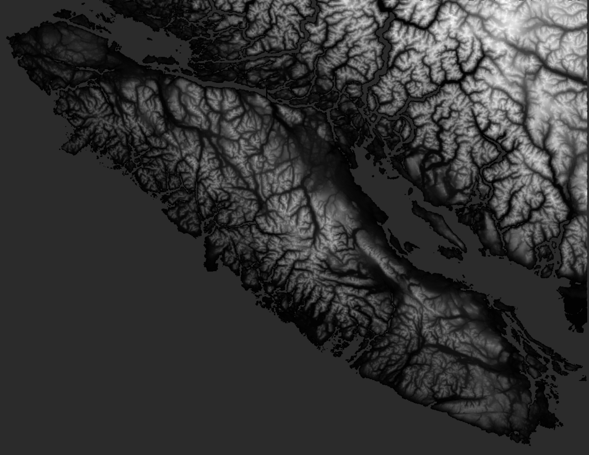
The HRDEM data for Vancouver Island, divided into a 4×5 grid of tiles for export
For this project, I exported the model as a 5x4 grid of tiles (14 of which Vancouver Island), with each tile sized to fit my printer's 256mm x 256mm build plate. The settings I used:
Model height:     12.1mm (vertical exaggeration 1.5x)
Base height:      2.0mm
Tile size:        256mm x 256mm
Resolution:       25m DEM
Output format:    Binary STL
Important: Record These Values
Make note of the input and output values from the DEMto3D plugin. You'll need them later to calculate the sea level threshold for colour separation.
The Problem: colour Separation at Sea Level
Here's where things got interesting. I wanted to print the ocean in black and the land in orange. Modern multi-colour printers like the Bambu P1S with AMS can swap filaments automatically, but they need to know which geometry belongs to which colour.
The naive approach would be to classify each triangle in the mesh: if it's below sea level, it's ocean; if it's above, it's land. But this creates a problem at the shoreline where triangles straddle the boundary.
Without geometry slicing, land triangles protrude down into what should be ocean-only layers

Without proper slicing, triangles that cross sea level cause excessive filament changes
A triangle that spans from -5m to +5m elevation has vertices both above and below sea level. If you classify the whole triangle as one material, you get incorrect colours. If you split based on the majority of vertices, you get a jagged, incorrect shoreline.
The Real Impact
Without proper geometry slicing, my test prints had many filament changes per layer, taking much longer to print and creating messy colour transitions along the coast. Not to mention a lot of wasted filament as the printer discards filament as part of the calibration process when switching colours.
The Solution: Boolean Geometry Slicing
The solution is to actually slice the geometry at the sea level plane. This means cutting triangles that cross the threshold and creating new vertices along the cut line. The Python trimesh library makes this surprisingly straightforward using boolean operations.

The mesh is intersected with bounding boxes above and below sea level
The algorithm:
- Calculate the sea level threshold in model space (mm)
- Create a bounding box from the bottom of the model to the threshold
- Create another box from the threshold to the top
- Intersect the original mesh with each box
- Result: two separate meshes with a clean horizontal cut
The Code
Here's the core slicing function from my Python script:
def slice_mesh_at_plane(mesh, threshold, verbose=False):
    """
    Slice mesh at horizontal plane (Z=threshold)
    Returns two meshes: ocean (below) and land (above)
    """
    import trimesh

    # Get mesh bounds for creating bounding boxes
    bounds = mesh.bounds
    margin = max(bounds[1] - bounds[0]) * 2

    # Create ocean bounding box (below threshold)
    ocean_box = trimesh.creation.box(
        extents=[margin, margin, threshold - bounds[0][2] + 1],
        transform=trimesh.transformations.translation_matrix([
            (bounds[0][0] + bounds[1][0]) / 2,
            (bounds[0][1] + bounds[1][1]) / 2,
            (bounds[0][2] + threshold) / 2 - 0.5
        ])
    )

    # Create land bounding box (above threshold)
    land_box = trimesh.creation.box(
        extents=[margin, margin, bounds[1][2] - threshold + 1],
        transform=trimesh.transformations.translation_matrix([
            (bounds[0][0] + bounds[1][0]) / 2,
            (bounds[0][1] + bounds[1][1]) / 2,
            (bounds[1][2] + threshold) / 2 + 0.5
        ])
    )

    # Boolean intersection to split the mesh
    ocean = mesh.intersection(ocean_box)
    land = mesh.intersection(land_box)

    return ocean, land
Calculating the Threshold
The threshold calculation maps real-world sea level (0m) to model coordinates (mm). This requires knowing the DEM's elevation range and the model's physical dimensions.
def calculate_threshold(config):
    """Calculate sea level threshold from DEM parameters"""
    params = config['dem_parameters']

    lowest = params['lowest_point_m']      # -220.726
    highest = params['highest_point_m']    # 3111.237
    base_height = params['base_height_mm']  # 2.00
    model_height = params['model_height_mm'] # 12.1
    offset = params.get('sea_level_offset_mm', 0.0)

    # Map 0m elevation to model Z coordinate
    threshold = (
        base_height +
        (abs(lowest) / (highest - lowest)) * model_height +
        offset
    )

    return threshold  # ≈ 2.82mm
I store these parameters in a JSON config file so I can reuse them across all tiles. These were all determined by the DEMto3D input settings and output values:
{
  "name": "vancouver_island_dem_25m",
  "dem_parameters": {
    "lowest_point_m": -220.726,
    "highest_point_m": 3111.237,
    "base_height_mm": 2.00,
    "model_height_mm": 12.1,
    "sea_level_offset_mm": 0.02
  }
}
Why OBJ Format?
After slicing the mesh into ocean and land portions, I needed an output format that preserves material information. STL files are geometry-only—they have no concept of materials or colours. OBJ format, however, supports material libraries (MTL files) that assign different materials to different parts of the mesh.

OBJ format preserves material assignments, enabling automatic colour separation in the slicer
The script generates an OBJ file with two material groups and an accompanying MTL file:
def write_obj_with_materials(ocean_mesh, land_mesh, output_path):
    # Write MTL file with material definitions
    with open(mtl_path, 'w') as f:
        f.write("newmtl Ocean_Material\n")
        f.write("Kd 0.0 0.5 1.0\n")  # Black

        f.write("newmtl Land_Material\n")
        f.write("Kd 0.6 0.4 0.2\n")  # Red

    # Write OBJ file with material assignments
    with open(obj_path, 'w') as f:
        f.write(f"mtllib {mtl_path.name}\n")

        # Ocean geometry with Ocean_Material
        f.write("usemtl Ocean_Material\n")
        # ... write vertices and faces

        # Land geometry with Land_Material
        f.write("usemtl Land_Material\n")
        # ... write vertices and faces
When Bambu Studio imports this OBJ file, it automatically recognizes the two materials and prompts you to assign filaments to each.

The Results
With properly sliced geometry, printing became dramatically more efficient. Each tile now has exactly one filament change per print—the swap from ocean to land that happens at sea level.
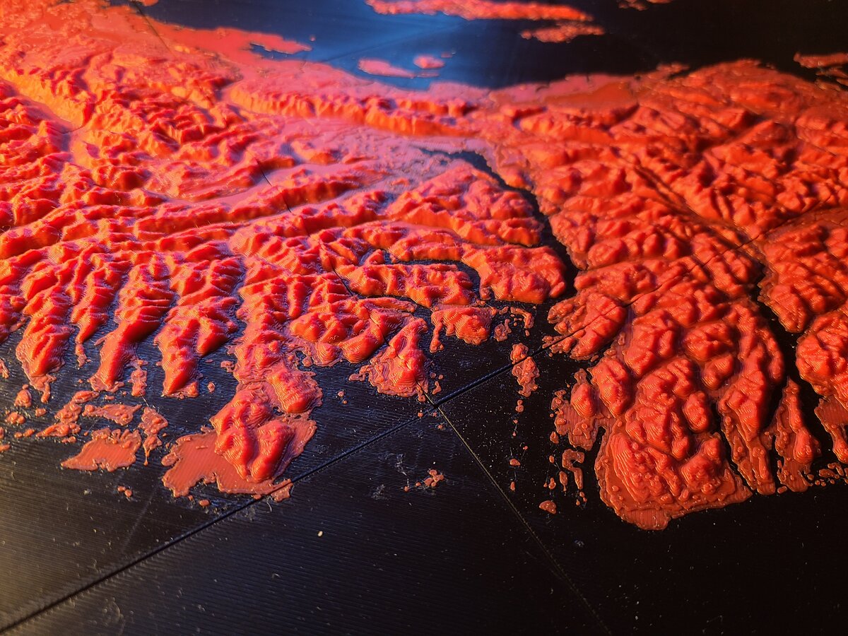
Inlet leading to Port Alberni.
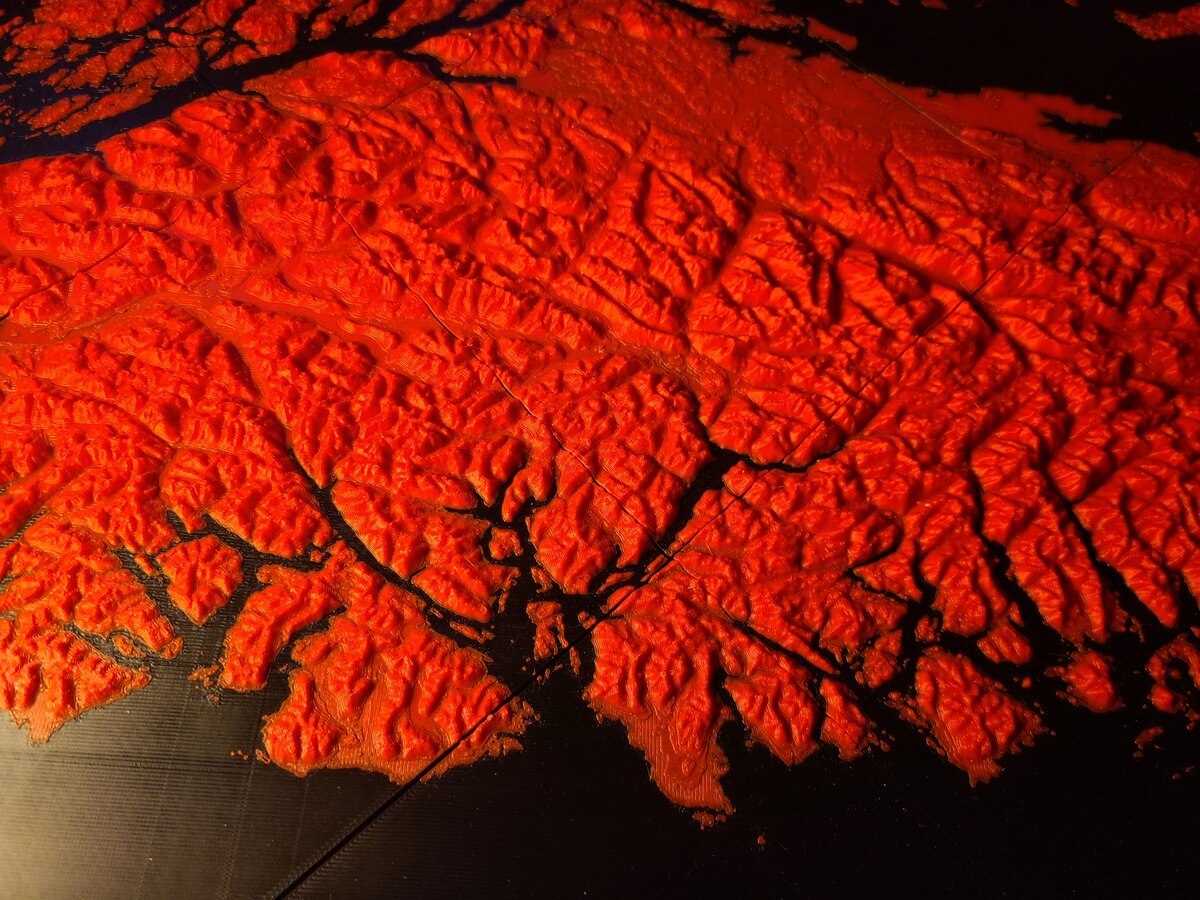
Central Island north of Port Alberni
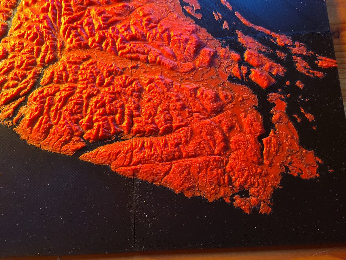
Victoria and the southern coast
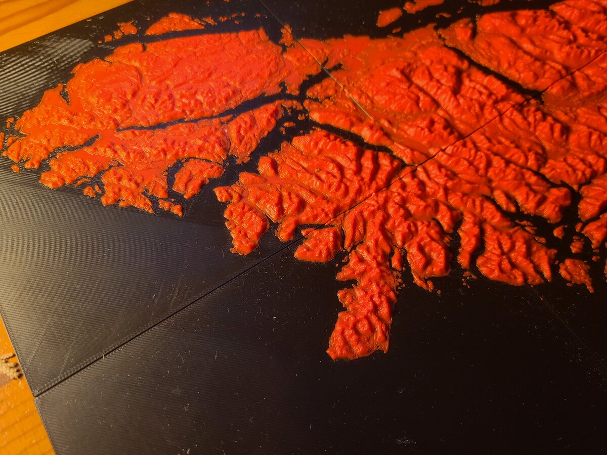
North Island
Print Statistics
| Metric | Value |
|---|---|
| Total tiles | 14 pieces |
| Print time per tile | ~3-4 hours |
| Layer height | 0.2mm |
| Filament changes per tile | 1 (at sea level) |
| Black filament (ocean) | ~400g total |
| Orange filament (land) | ~300g total |
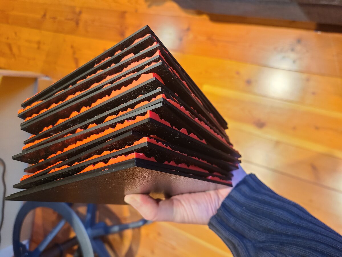
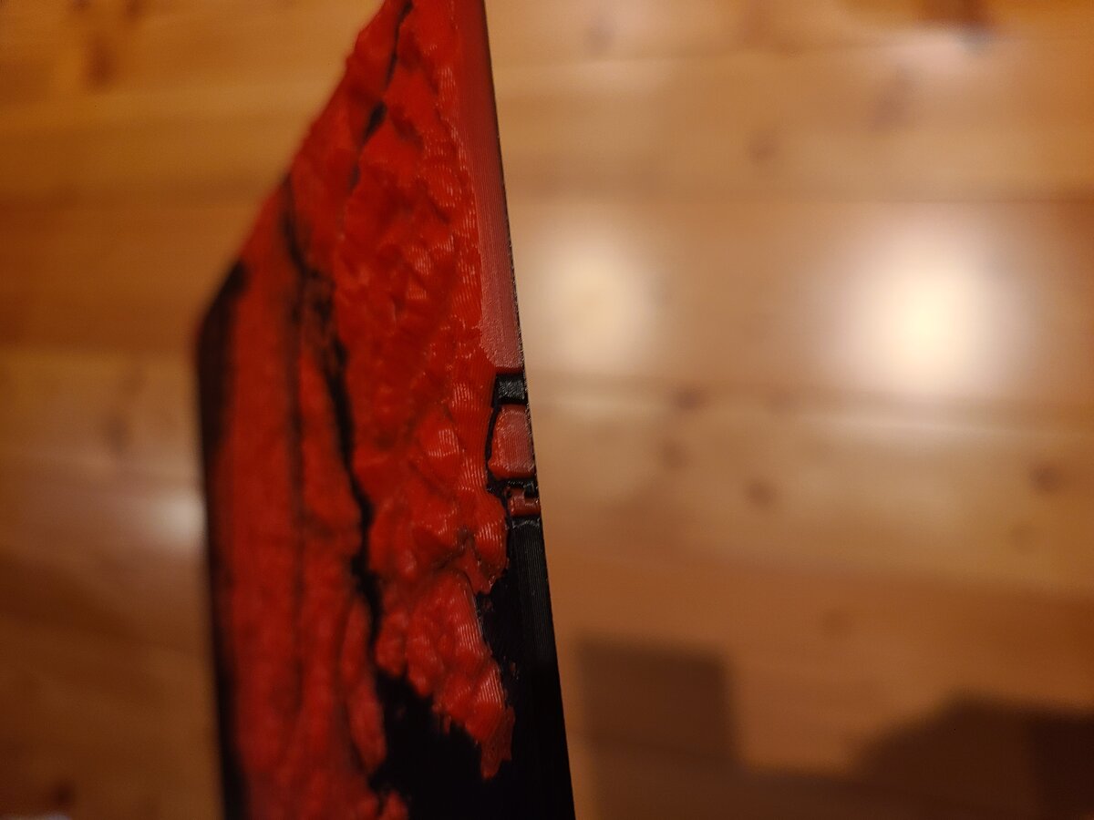
All 14 tiles stacked, showing the consistent sea level cut across pieces
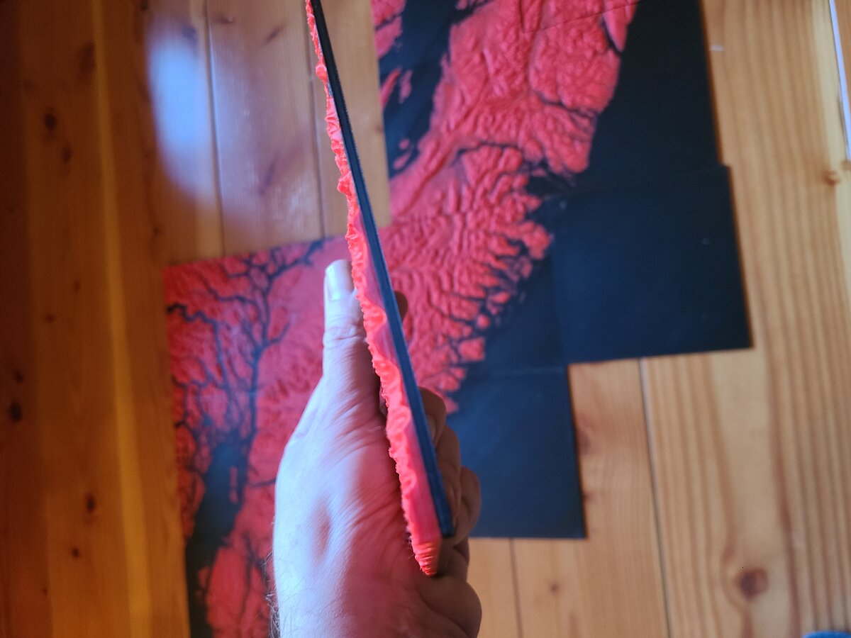
Side view showing the clean horizontal boundary between ocean (black) and land (orange)
Lessons Learned
Key Takeaways
Boolean mesh operations via trimesh are powerful and reliable. OBJ format is essential for multi-material printing. And vertical exaggeration makes terrain models much more dramatic.
- Boolean operations work: trimesh's mesh intersection is robust enough for production use. It handles the complex coastline geometry without issues.
- OBJ is the right format: For multi-colour printing, STL simply doesn't have the features you need. OBJ's material support maps perfectly to multi-material slicing.
- Config files matter: Storing DEM parameters in a config file ensures consistent processing across all tiles and makes it easy to adjust if needed.
- Vertical exaggeration is key: Real terrain is surprisingly flat at model scales. The 1.5x vertical exaggeration makes the mountains and valleys visible and dramatic.
- Test with one tile first: Always process and print a single tile before batch processing. It's much easier to adjust parameters on one file than to reprocess everything.
The Complete Model
Vancouver Island: from digital elevation data to physical terrain model
The finished model measures approximately 50cm x 100cm when all tiles are assembled. The black ocean provides excellent contrast against the orange land, and the terrain detail—from the rugged west coast fjords to the relatively gentle east coast—is clearly visible.
It's a satisfying project that combines several interests: GIS data processing, 3D printing, and a bit of computational geometry problem-solving.