Calculating Topographic Exposure with GRASS

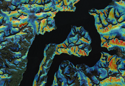
The goal of the analysis was to identify areas of low topographic exposure. The red areas illustrate low exposure.

Topographic exposure, also known as TOPEX, is a measure of the surrounding landforms and how they affect wind. This post shows how to generate a TOPEX model based on a digital elevation model. The tool of choice was GRASS, the free and extremely powerful open source GIS system.

What TOPEX Measures

Exposure is calculated based on the height and distance of the surrounding horizon. These two measures combine to form the angle of inflection. It is this angle that we use to quantify topographic exposure. When a large topographic feature, like a mountain, is far in the distance, the angle of inflection is low.

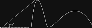
The angle of inflection is 45 degrees from the horizon.

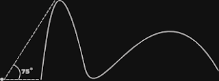
The angle of inflection is 75 degrees from the horizon.

When the same mountain is closer, the angle of inflection is higher. Therefore a higher angle of inflection equals lower exposure, or higher protection.

Based on advice from the windthrow expert Dr Stephen J. Mitchell, it was determined to calculate the angle of inflection at 100 metre intervals from 100 to 2000 metres. The maximum angle was then extracted to define the true value of exposure. This of course needs to be calculated for each cell within the raster dataset. Within GRASS this is accomplished with the r.mapcalc command.

Neighbour Calculations in GRASS

First, a little about neighbour calculations in GRASS. When we are looking at different spots on the horizon, we are essentially performing a neighbour function. The proper syntax for this is:

dem[3,1]

This translates into the raster cell three up and one to the right of the current cell. So if we wanted to subtract every cell in layer dem from the one that is three up and one to the right, it would look like this:

r.mapcalc newlayer = dem[3,1] - dem

Not sure why you'd want to do that… but there you go.

Building the TOPEX Equation

Now let's look at our topex equation. To calculate the angle of inflection we need to get the atan of the height difference divided by the distance. This was determined based on simple trigonometry. The GRASS equation looks like this:

r.mapcalc incl4north = "atan(((dem - dem[4,0])) / ((25 * 4)))"

This creates a layer incl4north which holds the angle of inclination for 4 cells to the north. Note we now need brackets around the equation. The dem and all subsequent raster layers have 25 metre cells. This is used to calculate the distance by multiplying by the number of cells. This one calculation creates a raster layer containing the exposure for 100 metres in just one direction.

Taking the Maximum Over All Distances

The goal is to take the maximum inclination for all distances from 100m to 2000m. Luckily there is a max() function for the r.mapcalc command. The following command calculates the maximum inclination for all intervals to the north:

r.mapcalc topex_n = "max(atan(((dem - dem[4,0])) / ((25 * 4))), \
atan(((dem[8,0] - dem)) / ((25 * 8))), \
atan(((dem[12,0] - dem)) / ((25 * 12))), \
atan(((dem[16,0] - dem)) / ((25 * 16))), \
atan(((dem[20,0] - dem)) / ((25 * 20))), \
atan(((dem[24,0] - dem)) / ((25 * 24))), \
atan(((dem[28,0] - dem)) / ((25 * 28))), \
atan(((dem[32,0] - dem)) / ((25 * 32))), \
atan(((dem[36,0] - dem)) / ((25 * 36))), \
atan(((dem[40,0] - dem)) / ((25 * 40))), \
atan(((dem[44,0] - dem)) / ((25 * 44))), \
atan(((dem[48,0] - dem)) / ((25 * 48))), \
atan(((dem[52,0] - dem)) / ((25 * 52))), \
atan(((dem[56,0] - dem)) / ((25 * 56))), \
atan(((dem[60,0] - dem)) / ((25 * 60))), \
atan(((dem[64,0] - dem)) / ((25 * 64))), \
atan(((dem[68,0] - dem)) / ((25 * 68))), \
atan(((dem[72,0] - dem)) / ((25 * 72))), \
atan(((dem[76,0] - dem)) / ((25 * 76))), \
atan(((dem[80,0] - dem) / ((25 * 80))))"

The Remaining Seven Directions

Now we need to do the same for the remaining seven directions: NE, E, SE, S, SW, W, and NW. East, south and west are simple — just rearrange the existing values. The remaining (diagonal) directions require a little more trigonometry. The hypotenuse is still the constant of 25 × (the number of cells). However, the remaining side of the triangle requires the following equation:

cos(45) * (25 * # cells)

I chose to calculate this in Perl with a function like this:

# Calculate one side of a right isosceles triangle.
sub is () {
    $value = floor(cos(deg2rad(45)) * $_[0]);
    return $value;
}

Then plug the function into the mapcalc command like this:

atan(((dem - dem[" . is(4) . "," . is(4) . "])) / ((25 * 4)))

This is just the way I decided to do it. You could use that same trigonometry formula however you choose.

Merging the Eight Directions

At this point we should have eight exposure raster layers. All that is required now is to merge them together, adding up the values. The command r.series does this beautifully:

r.series input=topex_n,topex_ne,topex_e,topex_se,topex_s,topex_sw, \
topex_w,topex_nw output=topex method=sum

Voilà! We now have a complete TOPEX layer… called topex.

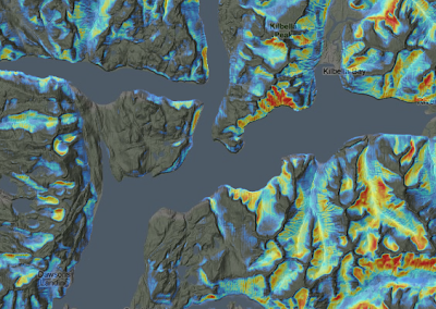
TOPEX highlighting areas of low exposure, draped over Google's Terrain basemap.

Exporting Beyond GRASS

To make use of the layer outside GRASS, I like to convert it to a GeoTIFF like this:

r.out.gdal -c input=topex createopt="COMPRESS=LZW" \
output=topex.tif nodata=0

If you have the GDAL library installed, you can also generate a pyramid on it like this:

gdaladdo topex.tif 2 4 8 16 32 64

Now the dataset can be moved around and consumed by most GIS software: ArcGIS, QGIS, GeoServer, and so on.

Jamie

← All Field Notes